Pipeline
1. Blocks cutting
1.1. Fetching data from OpenStreetMap.
The step can be skipped, if the data already exists.
[1]:
import osmnx as ox
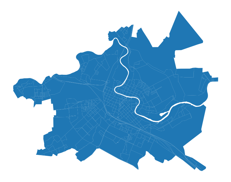
boundaries = ox.geocode_to_gdf('Санкт-Петербург, Василеостровский район')
boundaries.plot().set_axis_off()

[2]:
bc_tags = {
    'roads': {
      "highway": ["construction","crossing","living_street","motorway","motorway_link","motorway_junction","pedestrian","primary","primary_link","raceway","residential","road","secondary","secondary_link","services","tertiary","tertiary_link","track","trunk","trunk_link","turning_circle","turning_loop","unclassified",],
      "service": ["living_street", "emergency_access"]
    },
    'railways': {
      "railway": "rail"
    },
    'water': {
      'riverbank':True,
      'reservoir':True,
      'basin':True,
      'dock':True,
      'canal':True,
      'pond':True,
      'natural':['water','bay'],
      'waterway':['river','canal','ditch'],
      'landuse':'basin',
      'water': 'lake'
    }
}
[3]:
water = ox.features_from_polygon(boundaries.union_all(), bc_tags['water'])
roads = ox.features_from_polygon(boundaries.union_all(), bc_tags['roads'])
railways = ox.features_from_polygon(boundaries.union_all(), bc_tags['railways'])
[4]:
water = water[water.geom_type.isin(['Polygon', 'MultiPolygon', 'LineString', 'MultiLineString'])].copy()
roads = roads[roads.geom_type.isin(['LineString', 'MultiLineString'])].copy()
railways = railways[railways.geom_type.isin(['LineString', 'MultiLineString'])].copy()
[5]:
crs = boundaries.estimate_utm_crs()

for gdf in [water, roads, railways, boundaries]:
  gdf.to_crs(crs, inplace=True)
1.2. Preprocessing input geometry
The step can be skipped if input geometries are already sorted as lines, polygons and boundary.
[6]:
from blocksnet.blocks.cutting import preprocess_urban_objects, cut_urban_blocks

lines, polygons = preprocess_urban_objects(roads, railways, water)
2025-05-16 17:23:19.636 | INFO     | blocksnet.blocks.cutting.preprocessing.core:preprocess_urban_objects:36 - Checking roads schema
2025-05-16 17:23:19.674 | INFO     | blocksnet.blocks.cutting.preprocessing.core:preprocess_urban_objects:42 - Checking railways schema
2025-05-16 17:23:19.685 | INFO     | blocksnet.blocks.cutting.preprocessing.core:preprocess_urban_objects:48 - Checking water schema
1.3. Cutting urban blocks
[7]:
blocks = cut_urban_blocks(boundaries, lines, polygons)
2025-05-16 17:23:19.716 | INFO     | blocksnet.blocks.cutting.processing.core:wrapper:20 - Checking boundaries schema
2025-05-16 17:23:19.726 | INFO     | blocksnet.blocks.cutting.processing.core:wrapper:24 - Checking line objects schema
2025-05-16 17:23:19.741 | INFO     | blocksnet.blocks.cutting.processing.core:wrapper:30 - Checking polygon objects schema
2025-05-16 17:23:19.756 | INFO     | blocksnet.blocks.cutting.processing.core:_exclude_polygons:45 - Excluding polygon objects from blocks
2025-05-16 17:23:20.197 | INFO     | blocksnet.blocks.cutting.processing.core:_get_enclosures:51 - Setting up enclosures
2025-05-16 17:23:20.235 | INFO     | blocksnet.blocks.cutting.processing.core:_fill_holes:68 - Filling holes inside the blocks
2025-05-16 17:23:20.263 | INFO     | blocksnet.blocks.cutting.processing.core:_filter_overlapping:78 - Filtering overlapping geometries
2025-05-16 17:23:20.313 | SUCCESS  | blocksnet.blocks.cutting.processing.core:cut_urban_blocks:119 - Blocks are successfully cut!
[8]:
blocks.plot().set_axis_off()
2. Land use assignment
2.1. Fetching data from OpenStreetMap
The step can be skipped if functional zones layer is already obtained via goverment sources.
[9]:
import osmnx as ox

functional_zones = ox.features_from_polygon(boundaries.to_crs(4326).union_all(), tags={'landuse': True})
[10]:
functional_zones = functional_zones.reset_index(drop=True)[['geometry','landuse']].rename(columns={'landuse': 'functional_zone'})
functional_zones = functional_zones.to_crs(crs)
functional_zones.head()
[10]:
| geometry | functional_zone | |
|---|---|---|
| 0 | POLYGON ((345659.049 6646239.362, 345672.29 66... | commercial |
| 1 | POLYGON ((346755.014 6647579.789, 346728.91 66... | industrial |
| 2 | POLYGON ((345964.693 6646155.952, 346283.885 6... | industrial |
| 3 | POLYGON ((345753.722 6648393.897, 345900.252 6... | cemetery |
| 4 | POLYGON ((345900.252 6648481.707, 345896.076 6... | garages |
2.2. Specifying rules
Rules define how functional_zone column will be mapped into LandUse.
[11]:
from blocksnet.enums import LandUse

rules = {
  'commercial': LandUse.BUSINESS,
  'industrial': LandUse.INDUSTRIAL,
  'cemetery': LandUse.SPECIAL,
  'garages': LandUse.INDUSTRIAL,
  'residential': LandUse.RESIDENTIAL,
  'retail': LandUse.BUSINESS,
  'grass': LandUse.RECREATION,
  'farmland': LandUse.AGRICULTURE,
  'construction': LandUse.SPECIAL,
  'brownfield': LandUse.INDUSTRIAL,
  'forest': LandUse.RECREATION,
  'recreation_ground': LandUse.RECREATION,
  'religious': LandUse.SPECIAL,
  'flowerbed': LandUse.RECREATION,
  'military': LandUse.SPECIAL,
  'landfill': LandUse.TRANSPORT
}
2.3. Assignment
[12]:
from blocksnet.blocks.assignment import assign_land_use

blocks = assign_land_use(blocks, functional_zones.reset_index(drop=True).rename(columns={'landuse': 'functional_zone'}), rules)
2025-05-16 17:23:20.914 | INFO     | blocksnet.blocks.assignment.core:assign_land_use:44 - Overlaying geometries
2025-05-16 17:23:21.022 | SUCCESS  | blocksnet.blocks.assignment.core:assign_land_use:55 - Shares calculated
[13]:
blocks.head()
[13]:
| geometry | residential | business | recreation | industrial | transport | special | agriculture | land_use | share | |
|---|---|---|---|---|---|---|---|---|---|---|
| 0 | POLYGON ((345747.414 6646456.191, 345751.077 6... | 0.000000 | 0.000000 | 0.000000 | 0.0 | 0.0 | 0.000000 | 0.0 | None | NaN |
| 1 | POLYGON ((345751.077 6646449.404, 345747.414 6... | 0.000000 | 0.000000 | 0.000000 | 0.0 | 0.0 | 0.000000 | 0.0 | None | NaN |
| 2 | POLYGON ((345047.432 6648157.204, 345028.835 6... | 0.496234 | 0.093738 | 0.115348 | 0.0 | 0.0 | 0.000000 | 0.0 | LandUse.RESIDENTIAL | 0.496234 |
| 3 | POLYGON ((344951.065 6648110.08, 344977.865 66... | 0.000000 | 0.000000 | 0.000000 | 0.0 | 0.0 | 0.000000 | 0.0 | None | NaN |
| 4 | POLYGON ((346686.09 6647227.682, 346691.412 66... | 0.173093 | 0.116007 | 0.005135 | 0.0 | 0.0 | 0.167767 | 0.0 | LandUse.RESIDENTIAL | 0.173093 |
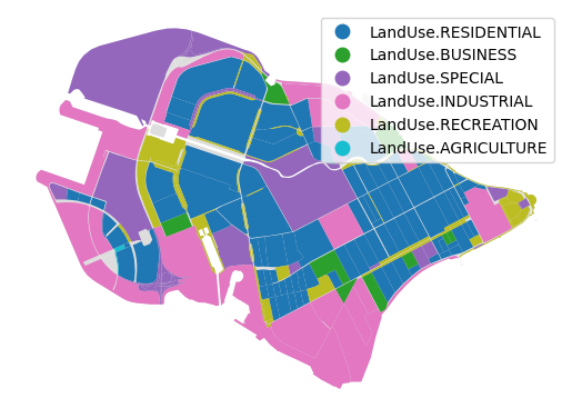
[14]:
ax = blocks.plot(color='#ddd')
blocks.plot(column='land_use', legend=True, ax=ax).set_axis_off()
3. Accessibility matrix calculation
There are few ways to define spatial relations between urban blocks: - Accessibility matrix – n^2 matrix that defines travel time between urban blocks’ centroids in minutes. - Distance matrix – n^2 matrix that defines euclidian distance between urban blocks’ centroids in meters. - Adjacency graph – graph with n nodes. Each edge of this graph indicates spatial adjacency of two urban blocks.
In this example the accessibility matrix will be calculated using IduEdu library.
3.1. Intermodal graph construction
There are few types of city graphs to model city network: - walk – pedestrian network. - drive – personal transport network. - intermodal – pedestrian and public transport network.
In this example intermodal graph will be constructed, but overall it depends on one’s research.
[15]:
from blocksnet.relations import get_accessibility_graph

graph = get_accessibility_graph(boundaries, 'intermodal')
2025-05-16 17:23:24.976 | WARNING  | blocksnet.relations.accessibility.graph:get_accessibility_graph:14 - CRS do not match IDUEDU required crs. Reprojecting
2025-05-16 17:23:24.978 | INFO     | iduedu.modules.drive_walk_builder:get_walk_graph:217 - Downloading walk graph from OSM, it may take a while for large territory ...
2025-05-16 17:23:52.489 | INFO     | iduedu.modules.pt_walk_joiner:join_pt_walk_graph:51 - Composing intermodal graph...
2025-05-16 17:23:55.362 | WARNING  | iduedu.utils.utils:remove_weakly_connected_nodes:37 - Removing 555 nodes that form 269 trap components. These are groups where you can enter but can't exit (or vice versa). Keeping the largest strongly connected component (20350 nodes).
3.2. Calculating the accessibility matrix
[16]:
from blocksnet.relations import calculate_accessibility_matrix

acc_mx = calculate_accessibility_matrix(blocks, graph)
[17]:
acc_mx.head()
/home/vasilstar/masterplanning/.venv/lib/python3.10/site-packages/pandas/io/formats/format.py:1458: RuntimeWarning: overflow encountered in cast
  has_large_values = (abs_vals > 1e6).any()
[17]:
| 0 | 1 | 2 | 3 | 4 | 5 | 6 | 7 | 8 | 9 | ... | 574 | 575 | 576 | 577 | 578 | 579 | 580 | 581 | 582 | 583 | |
|---|---|---|---|---|---|---|---|---|---|---|---|---|---|---|---|---|---|---|---|---|---|
| 0 | 0.000000 | 0.623535 | 13.679688 | 9.679688 | 7.523438 | 11.148438 | 18.71875 | 15.585938 | 17.484375 | 14.890625 | ... | 25.015625 | 13.789062 | 12.218750 | 13.820312 | 15.375000 | 14.859375 | 16.125000 | 21.109375 | 12.625000 | 20.078125 |
| 1 | 0.623535 | 0.000000 | 13.531250 | 9.531250 | 7.371094 | 10.992188 | 18.56250 | 15.437500 | 17.328125 | 14.742188 | ... | 24.859375 | 13.640625 | 12.070312 | 13.664062 | 15.218750 | 14.703125 | 15.976562 | 20.953125 | 12.468750 | 19.921875 |
| 2 | 13.398438 | 13.250000 | 0.000000 | 5.152344 | 17.250000 | 16.937500 | 19.37500 | 13.445312 | 15.343750 | 12.750000 | ... | 19.453125 | 11.640625 | 9.250000 | 11.679688 | 9.804688 | 9.281250 | 10.554688 | 17.046875 | 21.250000 | 15.898438 |
| 3 | 11.750000 | 11.593750 | 5.152344 | 0.000000 | 14.585938 | 14.187500 | 16.68750 | 10.742188 | 12.648438 | 10.046875 | ... | 18.562500 | 8.460938 | 7.371094 | 8.843750 | 8.921875 | 8.398438 | 9.671875 | 16.171875 | 19.250000 | 15.015625 |
| 4 | 7.953125 | 8.296875 | 17.281250 | 13.273438 | 0.000000 | 6.140625 | 16.90625 | 16.062500 | 15.890625 | 17.515625 | ... | 28.625000 | 17.390625 | 15.812500 | 17.421875 | 18.984375 | 18.453125 | 19.734375 | 24.718750 | 15.265625 | 23.687500 |
5 rows × 584 columns
4. Buildings aggregation
Buildings define the urban environment parameters in different blocks. For some blocksnet methods only population can be used, but overall the building is defined via:
population : floatfootprint_area : float– building’s base areanumber_of_floors : floatbuild_floor_area : float– sum area of each building flooris_living : boolliving_area : float– area defined for residentsnon_living_area : float– area not defined to live in
Some of these parameters may be optional, depends on what one already has.
4.1. Fetching data from OpenStreetMap
The step can be skipped if the data already obtained from any available source.
[18]:
buildings = ox.features_from_polygon(boundaries.to_crs(4326).union_all(), tags={'building': True}).reset_index(drop=True).to_crs(crs)
4.1.1. is_living
[19]:
is_living_tags = ['residential', 'house', 'apartments', 'detached', 'terrace', 'dormitory']
buildings['is_living'] = buildings['building'].apply(lambda b : b in is_living_tags)
4.1.2. number_of_floors
[20]:
import pandas as pd

buildings['number_of_floors'] = pd.to_numeric(buildings['building:levels'], errors='coerce')
4.2. Imputing missing data
[21]:
from blocksnet.preprocessing.imputing import impute_buildings

buildings = impute_buildings(buildings, default_living_demand=30)
2025-05-16 17:24:06.880 | WARNING  | blocksnet.preprocessing.imputing.buildings.schemas:_before_validate:21 - Column footprint_area not found and will be initialized as None
2025-05-16 17:24:06.881 | WARNING  | blocksnet.preprocessing.imputing.buildings.schemas:_before_validate:21 - Column build_floor_area not found and will be initialized as None
2025-05-16 17:24:06.881 | WARNING  | blocksnet.preprocessing.imputing.buildings.schemas:_before_validate:21 - Column living_area not found and will be initialized as None
2025-05-16 17:24:06.882 | WARNING  | blocksnet.preprocessing.imputing.buildings.schemas:_before_validate:21 - Column non_living_area not found and will be initialized as None
2025-05-16 17:24:06.882 | WARNING  | blocksnet.preprocessing.imputing.buildings.schemas:_before_validate:21 - Column population not found and will be initialized as None
[22]:
buildings.sample(5)
[22]:
| geometry | is_living | number_of_floors | footprint_area | build_floor_area | living_area | non_living_area | population | |
|---|---|---|---|---|---|---|---|---|
| 651 | POLYGON ((345707.15 6647277.813, 345713.366 66... | True | 5.0 | 1508.646392 | 7543.231961 | 6788.908765 | 754.323196 | 226.0 |
| 3767 | POLYGON ((347982.577 6648704.74, 347978.314 66... | False | 1.0 | 165.940125 | 165.940125 | 0.000000 | 165.940125 | NaN |
| 124 | POLYGON ((347167.301 6648613.826, 347159.307 6... | False | 1.0 | 2809.517622 | 2809.517622 | 0.000000 | 2809.517622 | NaN |
| 1126 | POLYGON ((346209.426 6646888, 346222.815 66468... | False | 1.0 | 364.041807 | 364.041807 | 0.000000 | 364.041807 | NaN |
| 1965 | POLYGON ((347965.1 6648464.713, 347967.454 664... | False | 1.0 | 56.805168 | 56.805168 | 0.000000 | 56.805168 | NaN |
[23]:
buildings.population.sum()
[23]:
np.float64(271251.0)
4.3. Aggregating buildings within blocks
[24]:
from blocksnet.blocks.aggregation import aggregate_objects

buildings_blocks = aggregate_objects(blocks, buildings)[0]
2025-05-16 17:24:07.003 | INFO     | blocksnet.blocks.aggregation.core:_preprocess_input:12 - Preprocessing input
2025-05-16 17:24:07.014 | INFO     | blocksnet.blocks.aggregation.core:aggregate_objects:41 - Aggregating objects
[25]:
buildings_blocks.head()
[25]:
| geometry | is_living | number_of_floors | footprint_area | build_floor_area | living_area | non_living_area | population | objects_count | |
|---|---|---|---|---|---|---|---|---|---|
| 0 | POLYGON ((345747.414 6646456.191, 345751.077 6... | 0.0 | 0.0 | 0.000000 | 0.000000 | 0.000000 | 0.000000 | 0.0 | 0.0 |
| 1 | POLYGON ((345751.077 6646449.404, 345747.414 6... | 0.0 | 0.0 | 0.000000 | 0.000000 | 0.000000 | 0.000000 | 0.0 | 0.0 |
| 2 | POLYGON ((345047.432 6648157.204, 345028.835 6... | 18.0 | 287.0 | 67273.384879 | 386154.823127 | 295058.918381 | 91095.904746 | 9827.0 | 72.0 |
| 3 | POLYGON ((344951.065 6648110.08, 344977.865 66... | 0.0 | 0.0 | 0.000000 | 0.000000 | 0.000000 | 0.000000 | 0.0 | 0.0 |
| 4 | POLYGON ((346686.09 6647227.682, 346691.412 66... | 1.0 | 32.0 | 3411.837763 | 54589.404201 | 24939.758056 | 29649.646145 | 831.0 | 2.0 |
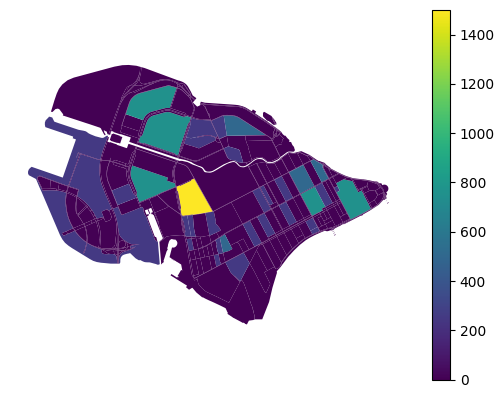
[26]:
buildings_blocks.plot('population', legend=True).set_axis_off()
5. Services aggregation
5.1. Fetching data from OpenStreetMap
And once again: if one already has the required data, the step can be skipped.
[35]:
schools = ox.features_from_polygon(boundaries.to_crs(4326).union_all(), tags={'amenity': 'school'}).reset_index(drop=True).to_crs(crs)
5.2. Imputing missing data
[36]:
from blocksnet.preprocessing.imputing import impute_services

schools = impute_services(schools, 'school')
[37]:
schools.head()
[37]:
| geometry | capacity | |
|---|---|---|
| 0 | POINT (345500.447 6647564.184) | 250.0 |
| 1 | POINT (348138.425 6647505.876) | 250.0 |
| 2 | POINT (348050.437 6648161.823) | 250.0 |
| 3 | POINT (346370.983 6648934.02) | 250.0 |
| 4 | POINT (348061.507 6648770.774) | 250.0 |
5.3. Aggregating services within blocks
[38]:
schools_blocks = aggregate_objects(blocks, schools)[0]
2025-05-16 17:28:03.882 | INFO     | blocksnet.blocks.aggregation.core:_preprocess_input:12 - Preprocessing input
2025-05-16 17:28:03.884 | INFO     | blocksnet.blocks.aggregation.core:aggregate_objects:41 - Aggregating objects
[39]:
schools_blocks.head()
[39]:
| geometry | capacity | objects_count | |
|---|---|---|---|
| 0 | POLYGON ((345747.414 6646456.191, 345751.077 6... | 0.0 | 0.0 |
| 1 | POLYGON ((345751.077 6646449.404, 345747.414 6... | 0.0 | 0.0 |
| 2 | POLYGON ((345047.432 6648157.204, 345028.835 6... | 750.0 | 3.0 |
| 3 | POLYGON ((344951.065 6648110.08, 344977.865 66... | 0.0 | 0.0 |
| 4 | POLYGON ((346686.09 6647227.682, 346691.412 66... | 0.0 | 0.0 |
[40]:
schools_blocks.plot('capacity', legend=True).set_axis_off()
6. Results
Using the methods above the following data can be obtained:
Urban blocks layer –
GeoDataFrameof urban blocks within the modeled territory (city).Land use assignment layer – the assignment of current land use according to any source of functional zones data.
Accessibility matrix –
DataFramen*nmatrix of accessibility values in minutes between each pair of urban blocks.Buildings aggregation layer – the aggregation of buildings parameters within urban blocks.
Services aggregation layer – the aggregation of services parameters within urban blocks.
It’s important to mention that any type of data can be aggregated within city blocks depending on the task.
7. Use examples
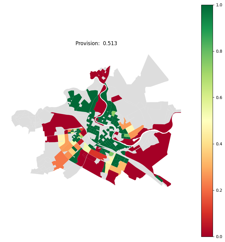
7.1. Competitive provision
[43]:
df = buildings_blocks[['population']].join(schools_blocks[['capacity']])
df.head()
[43]:
| population | capacity | |
|---|---|---|
| 0 | 0.0 | 0.0 |
| 1 | 0.0 | 0.0 |
| 2 | 9827.0 | 750.0 |
| 3 | 0.0 | 0.0 |
| 4 | 831.0 | 0.0 |
[49]:
from blocksnet.config import service_types_config

_, demand, accessibility = service_types_config['school'].values()
demand, accessibility
[49]:
(120, 15)
[51]:
from blocksnet.analysis.provision import competitive_provision

prov_df, links_df = competitive_provision(df, acc_mx, accessibility, demand)
2025-05-16 18:07:05.900 | INFO     | blocksnet.analysis.provision.competivive.core:_initialize_provision_df:29 - Initializing provision DataFrame
2025-05-16 18:07:05.901 | WARNING  | blocksnet.analysis.provision.competivive.core:_initialize_provision_df:33 - No demand in columns. Imputing using population column and demand parameter
2025-05-16 18:07:05.910 | INFO     | blocksnet.analysis.provision.competivive.core:_supply_self:56 - Supplying blocks with own capacities
2025-05-16 18:07:05.918 | INFO     | blocksnet.analysis.provision.competivive.core:competitive_provision:173 - Setting and solving LP problems until max depth or break condition reached
100%|██████████| 1/1 [00:00<00:00, 11.40it/s]
2025-05-16 18:07:06.009 | SUCCESS  | blocksnet.analysis.provision.competivive.core:competitive_provision:186 - Provision assessment finished
[57]:
prov_df.head()
[57]:
| demand | capacity | demand_left | demand_within | demand_without | capacity_left | capacity_within | capacity_without | provision_strong | provision_weak | |
|---|---|---|---|---|---|---|---|---|---|---|
| 0 | 0 | 0 | 0 | 0 | 0 | 0 | 0 | 0 | NaN | NaN |
| 1 | 0 | 0 | 0 | 0 | 0 | 0 | 0 | 0 | NaN | NaN |
| 2 | 1179 | 750 | 429 | 750 | 0 | 0 | 0 | 0 | 0.636132 | 0.636132 |
| 3 | 0 | 0 | 0 | 0 | 0 | 0 | 0 | 0 | NaN | NaN |
| 4 | 100 | 0 | 100 | 0 | 0 | 0 | 0 | 0 | 0.000000 | 0.000000 |
[58]:
links_df.head()
[58]:
| value | ||
|---|---|---|
| source | target | |
| 21 | 390 | 16.0 |
| 23 | 11 | 121.0 |
| 31 | 114 | 154.0 |
| 201 | 55.0 | |
| 59 | 213 | 76.0 |
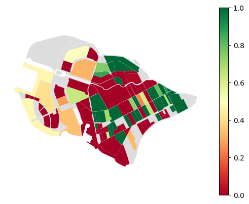
[56]:
ax = blocks.plot(color='#ddd')
blocks.join(prov_df).plot('provision_strong', ax=ax, cmap='RdYlGn', vmin=0, vmax=1, legend=True)
ax.set_axis_off()
7.2. Morphotypes
[63]:
from blocksnet.analysis.indicators import calculate_density_indicators

buildings_blocks['site_area'] = buildings_blocks.area
density_df = calculate_density_indicators(buildings_blocks)
density_df.head()
[63]:
| site_area | footprint_area | build_floor_area | living_area | non_living_area | fsi | gsi | mxi | l | osr | share_living | share_non_living | |
|---|---|---|---|---|---|---|---|---|---|---|---|---|
| 0 | 356.518194 | 0.000000 | 0.000000 | 0.000000 | 0.000000 | 0.000000 | 0.000000 | NaN | NaN | inf | NaN | NaN |
| 1 | 410.939744 | 0.000000 | 0.000000 | 0.000000 | 0.000000 | 0.000000 | 0.000000 | NaN | NaN | inf | NaN | NaN |
| 2 | 364393.913217 | 67273.384879 | 386154.823127 | 295058.918381 | 91095.904746 | 1.059718 | 0.184617 | 0.764095 | 5.740083 | 0.769434 | 4.385968 | 1.354115 |
| 3 | 4135.809669 | 0.000000 | 0.000000 | 0.000000 | 0.000000 | 0.000000 | 0.000000 | NaN | NaN | inf | NaN | NaN |
| 4 | 31474.102302 | 3411.837763 | 54589.404201 | 24939.758056 | 29649.646145 | 1.734423 | 0.108401 | 0.456861 | 16.000000 | 0.514061 | 7.309773 | 8.690227 |
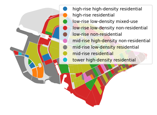
7.2.1. Spacematrix morphotypes
[65]:
from blocksnet.analysis.morphotypes import get_spacematrix_morphotypes

spacematrix_df, spacematrix_clusters = get_spacematrix_morphotypes(density_df)
[72]:
spacematrix_df.head()
[72]:
| l | fsi | mxi | cluster | morphotype | |
|---|---|---|---|---|---|
| 0 | 0.000000 | 0.000000 | 0.000000 | NaN | NaN |
| 1 | 0.000000 | 0.000000 | 0.000000 | NaN | NaN |
| 2 | 5.740083 | 1.059718 | 0.764095 | 7.0 | mid-rise residential |
| 3 | 0.000000 | 0.000000 | 0.000000 | NaN | NaN |
| 4 | 16.000000 | 1.734423 | 0.456861 | 2.0 | high-rise residential |
[73]:
spacematrix_clusters.head()
[73]:
| l | fsi | mxi | l_interpretation | fsi_interpretation | mxi_interpretation | morphotype | |
|---|---|---|---|---|---|---|---|
| cluster | |||||||
| 0 | 2.934850 | 1.154953 | 0.000000 | low-rise | None | non-residential | low-rise non-residential |
| 1 | 5.326747 | 1.748314 | 0.889017 | mid-rise | None | residential | mid-rise residential |
| 2 | 15.348045 | 1.679297 | 0.883299 | high-rise | None | residential | high-rise residential |
| 3 | 1.000000 | 0.035799 | 0.000000 | low-rise | low-density | non-residential | low-rise low-density non-residential |
| 4 | 3.450012 | 1.487791 | 0.568041 | mid-rise | None | residential | mid-rise residential |
[71]:
ax = blocks.plot(color='#ddd')
blocks.join(spacematrix_df).plot('morphotype', legend=True, ax=ax)
ax.set_axis_off()
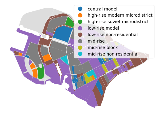
7.2.2. Strelka morphotypes
[74]:
from blocksnet.analysis.morphotypes import get_strelka_morphotypes

strelka_df = get_strelka_morphotypes(density_df)
[75]:
strelka_df.head()
[75]:
| l | fsi | mxi | morphotype | |
|---|---|---|---|---|
| 0 | 0.000000 | 0.000000 | 0.000000 | NaN |
| 1 | 0.000000 | 0.000000 | 0.000000 | NaN |
| 2 | 5.740083 | 1.059718 | 0.764095 | mid-rise |
| 3 | 0.000000 | 0.000000 | 0.000000 | NaN |
| 4 | 16.000000 | 1.734423 | 0.456861 | high-rise modern microdistrict |
[76]:
ax = blocks.plot(color='#ddd')
blocks.join(strelka_df).plot('morphotype', legend=True, ax=ax)
ax.set_axis_off()
7.3. Accessibility analysis
[85]:
from blocksnet.analysis.accessibility import area_accessibility

area_acc = area_accessibility(acc_mx, buildings_blocks)
[86]:
blocks.join(area_acc).plot('area_accessibility', legend=True).set_axis_off()